Up: Research Page
Also available in Postscript and DVI.
This paper has been examined and approved.
Examining Committee:






Artificial neural nets (ANNs) have been a tool to the artificial intelligence community since the 1960's. Numerous applications have since been found for these nets due to their ability to deal with dirty and incomplete data. Artificial neural nets have successfully been applied to problems as diverse as the diagnosis of medical problems and speech recognition [MP95]. Neural networks are generally used as classifiers to determine the membership of a given data instance in one group or another.
Neural networks are under-used, despite that the answers offered by such networks are statistically equal or better, when compared to those provided by other artificial intelligence constructs [Die92]. Neural networks are today used predominantly by researchers and academics. Outside of this realm, artificial neural nets are met with some skepticism due to the absence of explanation facilities [Die92]. Other artificial intelligence constructs, such as decision trees and genetic algorithms, provide their human users with explanations in the form of rules and probabilities, based on statistical analysis of the applicability of the given rule. Although neural networks are powerful tools which seem to perform well under many circumstances, their human users want an understanding of the results and not just a result.
This research examines a possible approach for the extraction of rule-based knowledge from artificial neural nets. An attempt is made to extract knowledge from neural networks by treating the networks as weighted directed graphs and partitioning the graphs based on graph theoretical properties.
Very little work has been done to find a means of extracting rules from neural nets. Much of the research into knowledge extraction from neural nets attempts to extract knowledge primarily through additional data structures and supplemental constructs instead of relying on the data and information stored in the neural net. The only alternative to the use of additional data structures discussed in the current literature is an exhaustive brute force method to extract such knowledge.
The extraction of knowledge from neural nets should be based directly on the neural net, since the addition of extra data structures may have an adverse impact on the rules found. Any approach to finding rules and knowledge in ANNs which draws only on the structure and information in the neural nets should therefore provide a cleaner set of answers and rules. Since neural nets provide statistically appropriate answers without the help of additional data structures, construction of rules encoded within the neural net should be based only on the network itself.
Artificial neural networks, also known as connectionist systems, are commonly described as ``massively parallel interconnections of simple neurons ...'' which collaborate to function as a larger unit [MP95]. In this sense, neural networks are not unlike parallel computers where many processors work together to perform a much larger task.
The individual processing elements in a neural network are commonly
known as neurons, perceptrons or cells. The function performed by
these neurons is the calculation of an activation value, which
consists of the summation of its inputs. The output of a neuron is
discrete (with values of
 or
or
 ) or continuous (with values in a range such as
![$\left[0,1\right]$](img13.png) ,
,
![$\left[-1,1\right]$](img14.png) or
or
![$\left[-0.5,0.5\right]$](img15.png) ),
but is always bounded. This bounding necessitates an adjustment of
the activation value to satisfy the range or value requirement placed
on the activation values. Sigmoid or Gaussian functions are commonly
used to achieve this adjustment. Typically, each neuron in a neural
network uses the same function for this adjustment.
),
but is always bounded. This bounding necessitates an adjustment of
the activation value to satisfy the range or value requirement placed
on the activation values. Sigmoid or Gaussian functions are commonly
used to achieve this adjustment. Typically, each neuron in a neural
network uses the same function for this adjustment.
The activation value is then passed to the next neuron via a weighted connection. The weight of the connection is used to multiply the output of a neuron before it is input to the next neuron. Thus, positive weights indicate a reinforcement of the activation value, whereas negative weights inhibit the effects of the given activation value.
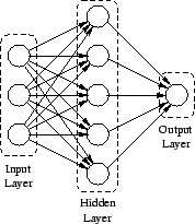
The neurons in the neural net are partitioned into three layers: input, output, and hidden. The information enters the network at the input layer. The number of input neurons is therefore the same as the number of variables in the data set. Since the values of the variables in the data set may very well differ from the acceptable range or values for a neurons activation values, there may be a need to pre-process the input variables to fit within the acceptable range or values.
The output layer is where the neural net produces its answer or classification. The output layer must have at least one output node, but may very well have several, depending upon the complexity and nature of the problem presented.
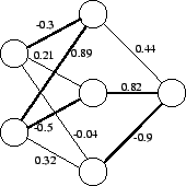
It is in the hidden layer where the actual computation takes place. Unlike the input and output layers, of which there is only one each, there may be more that one hidden layer. Figure 1 shows a small neural net. Neural nets are, in general, much larger than the one shown in order to allow for a possibly large amount of knowledge to be distributed across the entire artificial neural net.
Before neural nets are usable they must be trained. This is done by presenting sample data to the network in the form of a test set which includes the desired output. The weights in the network are adjusted if the produced result does not match the expected output and left unchanged if the result was correct. The training process continues until the rate of error is acceptable, which is determined by the problem domain and the user of the neural net. Thus, the acceptable rate of misclassification for a problem upon which lives depend will be much smaller than the acceptable error rate for the optimal usage of dinner ingredients.
After training is complete, the network is tested with a test set. The test set differs from the training set to ensure that the network performs as expected on data outside of the training set. Careful attention must be paid to obtain a properly trained neural net able to handle data from across the entire problem domain. Both under- and over-training are undesirable. Under-training results when the training data are presented to the neural net too few times, leading to higher error rates. Over-training occurs when the network becomes to closely attuned to the training data. This manifests itself by providing low error rates for instances from the training set, but a much higher rate of misclassification for instances from outside the training set.
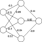
The structure of neural nets is very similar to that of weighted directed graphs or digraphs. The nodes in the neural nets become vertices in the digraphs. The neural net's connections become the weighted edges of the graph. By using the weights of the connections it is possible to treat a given neural net as a weighted digraph. The terms net, graph and digraph are used interchangeably throughout, as are edge and connection. Figure 2 shows a small neural net and the weights on its connections.
Although the normal path of travel followed by data through a neural net after training is unidirectional from the input nodes to the output node(s), it is it is possible to use the weights as a direction indicator. Positive weights indicate direction from input toward output and negative weights are directed from the output toward the input.
For the purpose of this research only feed-forward back-propagation neural nets are considered. Feed-forward means that, during the classification process data are only fed forward through the network, and there are no cycles which provide feedback to an earlier neuron. Back-propagation is the method of training, where the adjustments of connection weights, due to misclassification of training instances, are propagated backwards through the neural net. Note that back-propagation does not stand in contradiction to a definition of feed-forward, since the back-propagation during training does not affect the classification process which only uses feed-forward.
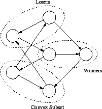
The graph structures examined in this research are convex subsets,
directed vertex covers, and spanning trees. A convex subset is a
subset of vertices such that each vertex not in the subset either
dominates or is dominated by all vertices within the convex subset. A
vertex  is said to dominate another vertex
  if there exists an
edge leading from to . All 2-paths between vertices in the
same convex subset are completely contained within that convex subset.
In other words, it is impossible to begin at a vertex inside the
convex subset, then leave and immediately re-enter the subset with
only two hops across edges. The vertices which dominate all vertices
in the convex subset are called winners, whereas those dominated by
the vertices in the convex subset are the losers.
Figure 3 provides an example of the relationships among
convex subset, winners and losers.
if there exists an
edge leading from to . All 2-paths between vertices in the
same convex subset are completely contained within that convex subset.
In other words, it is impossible to begin at a vertex inside the
convex subset, then leave and immediately re-enter the subset with
only two hops across edges. The vertices which dominate all vertices
in the convex subset are called winners, whereas those dominated by
the vertices in the convex subset are the losers.
Figure 3 provides an example of the relationships among
convex subset, winners and losers.
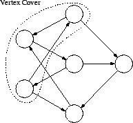
A directed vertex cover is a set of vertices such that each vertex not in the cover is dominated by at least one vertex inside the directed vertex cover. In general, the smallest vertex cover is sought. In this research however, all directed vertex covers are considered to allow for greater diversity in the potential rules extracted. An example of such a structure is provided in Figure 4.
A spanning tree is defined as a collection of edges without cycles, providing exactly one path from each vertex to every other vertex in the graph. Two types of spanning trees are considered in this research. The first type of spanning tree consists of the maximum weight edges, and the second type is based on the minimum non-zero weights. For both types of spanning trees all edge weights are treated as absolute values by eliminating the signs for all weights and using only the remaining absolute value. This leads to the largest (positive or negative) weights comprising the maximum weight spanning tree, and the smallest non-zero (positive or negative) weights to be part of the minimum weight spanning tree. Figure 5 shows a maximum absolute weight spanning tree.
The literature dealing with knowledge extraction form artificial neural networks is sparse. A search for available research revealed only three previously studied methods for extracting knowledge from neural nets.
The first method of knowledge extraction from neural nets is network inversion. This method of knowledge extraction is a brute force approach and works in the following way [Ebe92].
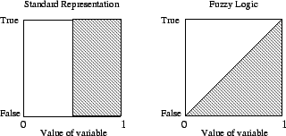
The algorithm discussed in [HNY96] uses fuzzy logic to provide an explanation facility for neural networks. Narazaki et al. describe the application of fuzzy logic to a logical formula as the extension of a truth value to a real number. For example, given the height of a person we can classify the individual as either ``tall'' or ``not tall'' using traditional sets. There is no different description for people who are somewhat tall. Fuzzy sets remedy this by providing degrees of membership[PT92]. Figure 6 illustrates how fuzzy sets provide much finer granularity in the classification process.
At the heart of the approach discussed in [HNY96] lies a
partitioning of the input space  into monotonic regions. The
membership in a monotonic region
into monotonic regions. The
membership in a monotonic region  depends on two conditions.
First, any two input vectors in must be classified the same by the
neural net, and second they must have the same sensitivity pattern.
The sensitivity pattern of an input vector
depends on two conditions.
First, any two input vectors in must be classified the same by the
neural net, and second they must have the same sensitivity pattern.
The sensitivity pattern of an input vector  is given as follows

 is the output of the neural network,
  is the size of the input
vector, and the function
is the size of the input
vector, and the function  returns '
 ' if the value examined
is greater or equal than
' if the value examined
is greater or equal than  and '
and ' ' if it is strictly less than
. These patterns of ''s and ''s are used to group the
training instances and provides the fuzzy structure needed for the
rule production. The sensitivity patterns can be generated using the
same input vectors used to train the network.
' if it is strictly less than
. These patterns of ''s and ''s are used to group the
training instances and provides the fuzzy structure needed for the
rule production. The sensitivity patterns can be generated using the
same input vectors used to train the network.
The above process divides the input space into a set of monotonic
regions
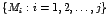 . Rules are then
generated by projecting each monotonic region
. Rules are then
generated by projecting each monotonic region  onto each variable
domain, which yields rules such as ``If
onto each variable
domain, which yields rules such as ``If  is approximately
 , and
, and  is approximately
  ,
,  , and
, and  is
approximately
is
approximately  , then it belongs to class
  , where is one
of the classes of the problem domain and
, where is one
of the classes of the problem domain and
 are the coordinates of the center of the monotonic
region .
are the coordinates of the center of the monotonic
region .
It is interesting to note that while this algorithm does provide an explanation facility via rule extraction, it does not provide the same accuracy as a decision tree. According to [HNY96] the algorithm is an approximation since there is a trade-off between readability and accuracy. The authors give the example that
we say ``Birds fly'', knowing that there is at least one bird(e.g. a penguin) that does not fly. In this example, that accuracy gives way to the simplicity of the knowledge description to a certain degree, and the occurrence of exceptions is allowed.
Genetic algorithms can also be the foundation for an explanation facility in neural networks [ED91]. Genetic algorithms attempt to model the evolutionary behavior of biological systems [NS92]. The operators used by genetic algorithms are reproduction, crossover and mutation and the genetic material used in this research consists of the input vectors to the neural network. Reproduction is used to preserve input vectors between evolutionary cycles. Crossover produces a new vector by combining parts of two different input vectors. The last operator is mutation and serves the purpose of preventing the pool of input vectors from evolving into a dead end. Although mutation may eliminate desirable input vectors as well as disposing of unwanted input vectors, it is very useful in keeping the evolutionary process going. The overall performance of the genetic algorithm is controlled by a fitness function, which determines the goodness of a given genetic string. In this research the neural net acts as the fitness function by comparing the actual output to the expected output and using this to determine the fitness of a given input vector. This fitness value is then used to determine which genetic operator is to be applied to the given vector.
A neural net's input domain can be viewed as a multi-dimensional space where each input vector represents a point in this space. Genetic algorithms are used in finding points on the decision hyper-surface within this space of the neural net's input domain. This decision hyper-surface provides the separation of one classification from another. Alternatively, by connecting the points found by the genetic algorithm we find that the input vectors above the curve are members of one classification and those below the curve are members of another classification.
Eberhardt[Ebe92] does not offer an actual mechanism for
rule extraction. However, it is clear that once the input space is
mapped, only a partitioning process is needed to group the points.
The groupings can then be used to extract rules. For example we find
the minimum and maximum values for each variable within a grouping to
generate rules of the form

Another point of interest is that this technique may also be used to generate additional training samples for partially trained neural nets, if only few training samples are available. This generation of additional training instances is done by searching out borderline instances through the use of genetic algorithms and then presenting the instances close to the activation value to an expert. After the expert classifies the instance it can be used as part of the training set.
In order to examine the graph structures in neural nets, several such networks are trained and searched for the presence of convex subsets, directed vertex covers, and spanning trees. The neural net package used is NevProp4 developed at the University of Nevada, Reno [Goo]. This package offers the back-propagation, configuration and output features necessary for the research at hand, while being very fast and simple to use.
In order to evaluate the usefulness of the graph theoretical properties considered in this research, a number of different neural nets are trained. The resulting network weight files are then treated as weighted digraphs. If knowledge extraction is possible through the use of convex subsets, directed vertex covers, or spanning trees, then it should be possible to find certain characteristics which hold true across different neural nets. For example, the absence or presence of overlapping convex subsets, within a single digraph, may indicate a logical OR, convex subsets which share no vertices may point towards a logical NEGATION. Thus, the primary focus in this research lies in the search for similarities and differences which point toward possible rules.
In order to determine how the presence and structure of graph theoretical properties relates to potential rules, different neural nets are compared to one another. The basis for the comparison is the degree of similarity between the properties found in different neural nets. It is expected that neural networks trained with similar data, and encoding similar knowledge, also share some low-level graph properties.
Generally, graphs and sub-graphs are not compared based on the labels of their vertices, since this labeling is arbitrary. However, in this research the labeling of the vertices is fixed and crucial to the results. The size of all neural nets used in this research is a direct function of the number of input variables, and therefore the numeric label assigned to a vertex also denotes the function of the vertex. For example, the highest numbered vertex is always the output node, whereas the vertices with the smallest numeric labels always serve as input.
As an additional note, it must be pointed out that the properties used in this research do not necessarily improve upon the performance of even the brute force network inversion discussed in Chapter II. The search for all directed vertex covers, for example, requires exponential running time. However, if directed vertex cover is useful in the extraction of knowledge from neural nets, then there may be some optimization that can be used with respect to this problem, to improve upon the efficiency of the approach.
The tools needed for the generation of test data and the extraction of graph structures from the trained networks are custom developed for this research. The graph extraction tools perform no evaluation or filtering of the data found. Several trained networks are used to compare the graph structures found and search for possible correlations between different networks. Similarities and differences are potential indicators of rules.
For example, it is possible that for the graphs derived from boolean expressions with a high degree of similarity there will be a high degree of overlap among convex subsets of each of the graphs. It may also be that case that overlapping and disjoint graph properties in a single network indicate the operators of the boolean expression used during training. More precisely, the overlapping substructures in a neural net may indicate a conjunction or logical AND, while completely separate substructures could point towards a disjunction or logical OR.
The test data for this research consist of truth tables based on
boolean expressions.
In order to gain a good understanding, care is taken to use a number of different expressions. The first four expressions in Table 1 use two distinct variables. The next four expressions are based on three variables each. The last two expressions have four input variables. Although these last two expressions are technically based on only two variables, it was necessary to treat each occurrence of a variable as a separate input in order to properly train the network. Proper training of a neural network depends on the application and the acceptable margin of error. In this research proper training is assumed to be perfect classification of all training data.
Expression  in Table 1 is based on the XOR
operator, but expressed using only the operators AND,
OR and NEGATION. The truth table based on
XOR operator failed to train the network without errors, and
always misclassified some of the training and testing instances. The
re-written expression, however, manages to achieve proper training of
the network, with perfect classification of all training and testing
data, when four distinct input variables are used. Expression
in Table 1 is based on the XOR
operator, but expressed using only the operators AND,
OR and NEGATION. The truth table based on
XOR operator failed to train the network without errors, and
always misclassified some of the training and testing instances. The
re-written expression, however, manages to achieve proper training of
the network, with perfect classification of all training and testing
data, when four distinct input variables are used. Expression  ,
the complement of expression , is present to allow a point of
comparison for expression . Each occurrence of the variables
will be fed to a different input node of the neural network and, thus,
require four input nodes.
,
the complement of expression , is present to allow a point of
comparison for expression . Each occurrence of the variables
will be fed to a different input node of the neural network and, thus,
require four input nodes.
Several tests are used to examine potential opportunities for rule extraction from neural nets.
 and
and  , both use
conjunctions, it is expected that there exists some degree of
overlap in the convex subsets, directed vertex covers and spanning
trees found in the digraphs based on those expressions.
, both use
conjunctions, it is expected that there exists some degree of
overlap in the convex subsets, directed vertex covers and spanning
trees found in the digraphs based on those expressions.
 and
and  use disjunctions and should
therefore contain a low level of overlap of convex subsets, directed
vertex covers and spanning trees.
and
is expected to produce very little overlap of convex subsets,
directed vertex covers and spanning trees.
and should generate some
low level of overlap in the convex subsets, directed vertex covers
and spanning trees found.
and is expected to yield
very little overlap in convex subsets, directed vertex covers and
spanning trees since their respective operators very greatly.
and due
to the significant differences between them.
use disjunctions and should
therefore contain a low level of overlap of convex subsets, directed
vertex covers and spanning trees.
and
is expected to produce very little overlap of convex subsets,
directed vertex covers and spanning trees.
and should generate some
low level of overlap in the convex subsets, directed vertex covers
and spanning trees found.
and is expected to yield
very little overlap in convex subsets, directed vertex covers and
spanning trees since their respective operators very greatly.
and due
to the significant differences between them.
 and
and  are expected to have a
significant overlap of convex subsets, directed vertex covers and
spanning trees, since the expressions only differ in one operator.
are expected to have a
significant overlap of convex subsets, directed vertex covers and
spanning trees, since the expressions only differ in one operator.
 and
and
 should result in very low overlap of convex subsets, directed
vertex covers and spanning trees
and are complements of one another and as such are
expected to have very little overlap of convex subsets, directed
vertex covers and spanning trees.
should result in very low overlap of convex subsets, directed
vertex covers and spanning trees
and are complements of one another and as such are
expected to have very little overlap of convex subsets, directed
vertex covers and spanning trees.
In order to minimize the size and thus the complexity of the ANNs
several tests were conducted to determine the smallest networks that
can properly classify the entire training set. These tests show that
at least  nodes are necessary, where
  is the number of input
nodes to the neural net. This calculation yields a network
configuration with input nodes, hidden nodes and one output
node. As mentioned earlier, each occurrence of a variable in a
boolean expression requires its own input node. Another result of
these preliminary tests is that each neural net must be trained by
presenting it with the training and testing data
is the number of input
nodes to the neural net. This calculation yields a network
configuration with input nodes, hidden nodes and one output
node. As mentioned earlier, each occurrence of a variable in a
boolean expression requires its own input node. Another result of
these preliminary tests is that each neural net must be trained by
presenting it with the training and testing data  times. Using
this number of iterations results in the perfect classification of all
training and testing data for each of the neural nets. Perfect
classification in this case means that the neural net makes no
mistakes given the testing or training data.
times. Using
this number of iterations results in the perfect classification of all
training and testing data for each of the neural nets. Perfect
classification in this case means that the neural net makes no
mistakes given the testing or training data.
While it is generally necessary to split the available data into two independent sets to verify that the network can handle data other than that contained in the training set, this is not necessary here. Since all data for the problem are available, all data, or the entire truth table, is used for both training and testing. This choice of training and testing data also averts the problem of over-training in which the network is able to handle only the training and not the testing datasets, which in this case are identical.
To further make the neural nets more uniform a full connection
model is chosen. Fully connected with respect to neural nets means
that each node on a given layer is connected to all nodes on the
following layer. No connections exist between nodes of the same
layer. During testing all neural nets had their weights initialized
to to further level the playing field between the different nets.
In general, comparing digraphs based on their vertex labels is not
practical. In this research however, the label is of significance
since it describes the function of the vertex. For example, the
highest numbered vertex is always the output node of the neural net,
whereas the lowest numbered vertices are those receiving input.
This observation is also relevant when considering that any
potentially generated rules must be somehow related to the problem
domain. The only means of doing so is in relying on input and output
nodes. It is for this reason that the labeling is considered to be
fixed: identical vertex subsets from different digraphs are treated as
identical when comparing properties of those digraphs. For example,
the subset
 occurring in two digraphs of equal
size are considered to be identical for the purpose of this research.
occurring in two digraphs of equal
size are considered to be identical for the purpose of this research.
In order to find the convex subsets, the neural nets are treated as digraphs, where the direction of a given edge is dependent upon the sign of its weight. A negative weight is interpreted as flowing in the opposite direction of the normal ANN from-input-to-output layer path. The convex subsets are used to compare the digraphs to one another. The digraphs based on similar boolean expressions are examined for an overlap in the sets of convex subsets. A small overlap is expected for digraphs based on expressions with similar features, such as conjunction, negation and number of variables.
and
, and
and
.
A comparison between the convex subsets found for neural networks
trained with truth tables from different boolean expressions yields
two sets with identical convex subsets. These sets are found in the
digraphs based on the expressions
and .
The expression
and
the XOR expression
also yields the exact same set of convex subsets, but the
sets of winners and losers differ in this case. A full listing of the
convex subsets found for each of the neural nets is available in
Appendix A.
In the search for potential directed vertex covers, the ANN is treated
similarly to the case of the convex subsets. Again, the natural
direction of the edges is reversed if the given weight of the edge is
negative. All digraphs produced numerous directed vertex covers. The
tests are centered around a comparison of the directed vertex covers
found for different digraphs. The overlap in the directed vertex
covers is examined based on the similarity of the boolean expressions
used in the creation of the neural net. The occurrence of similar
operators, such as conjunction and disjunction, as well as negation
and the number of variables, are examined for the presence of overlap
in the vertex covers discovered. As is the case with the convex
subsets, attention is also paid to the effect which operators and the
number of variables have on the overall number of directed vertex
covers discovered.
and yield the exact same set of directed vertex covers. The
expressions compared in Table 5 are
identical to those in Table 3. The pairing of
similar expressions in Table 5 shows that
those expressions with conjunctions and/or negation produce at least
as many directed vertex covers as the expression which lack negation
or use disjunctions.
In the search for spanning trees the sign of an edge weight is
ignored, since it does not directly affect the flow in the neural net
and forcing the search to honor the sign can potentially affect the
presence of a spanning tree. Using the absolute values of the weights
it is possible to direct the search towards an overall activation
value. The activation value has a direct affect on how strongly or
subtly the output of a neuron or vertex is changed. For this reason
two searches are conducted for both the spanning tree with the
smallest combined non-zero edge weight and for the largest combined
edge weight. The degree of overlap between the spanning trees for
different digraphs is examined as a possible indicator of knowledge.
Unlike the test for convex subsets and directed vertex covers, the
affect on the size of the set found is ignored, since the size of the
spanning tree is fixed based on the size of the digraph.
Table 6 and Table 7
show the number of edges common between the maximum and minimum
spanning trees respectively. The expressions based on two variables
produce digraphs with five vertices. The number of edges for the
spanning tree in such digraphs is thus four.
Table 6 shows that the digraphs based on the
expressions ,
, and
have identical maximum spanning trees. The
minimum spanning tree for the expressions and
are also identical according to the data presented in
Table 7.
The number of edges needed for a spanning tree in the 3-variable
expressions is six given that there are  vertices. The overlap
in spanning trees in digraphs based on 3-variable expressions are
shown in Table 8 and
Table 9. In this set of digraphs there are no
identical maximum or minimum spanning trees between the different
digraphs.
vertices. The overlap
in spanning trees in digraphs based on 3-variable expressions are
shown in Table 8 and
Table 9. In this set of digraphs there are no
identical maximum or minimum spanning trees between the different
digraphs.
The expression
and
the XOR expression
exhibited a perfect match for the maximum spanning tree
as illustrated in Table 10. However, the
minimum spanning trees for those expressions differed, as illustrated
in Table 11.
There are a number of trends which are apparent across the data
collected on convex subsets and directed vertex covers. For example,
that presence of negation and conjunction appears to increase the
number of convex subsets found in the digraph. This trend is reversed
with respect to directed vertex covers, where the lack of negation and
disjunction yields a more simplified graph in terms of the number of
directed vertex covers. A notable exception to these trends is the
expression
, which provided the smallest number of
directed vertex covers.
The presence of identical convex subsets and directed vertex covers
for the expressions
and is a strong
indication that neither of these two approaches offer a great hope for
the extraction of knowledge from neural nets, since it is impossible
to distinguish between the two expressions. Given that the
expressions are identical from the perspective of convex subset and
directed vertex cover, it is impossible to extract rules to reflect
the different original expressions.
The spanning trees approach also provided identical matches for the
expressions ,
, and
as well as and
. For the
first group, the maximum spanning tree was identical among all three
digraphs, and the second group of expressions shared the minimum
spanning tree in common. This again renders these approaches
ineffective as means of knowledge extraction from neural nets for the
aforementioned reasons.
A brief examination of the weights produced by the neural net package, which is provided in Appendix A, shows that the weights appear to occur in pairs of similar absolute values. This symmetry is most likely due to the dichotomous nature of the input used and raises some additional doubts about the usefulness of the spanning tree approach.
Overall it appears that the structure of the neural network alone is not enough to extract rules from a neural net. The performance of convex subsets and directed vertex covers are likely suffering because they fail to consider the actual weight of the edges beyond the sign. However, even the spanning tree approach did not produce unique data for each expression, despite taking the weights into consideration. The performance of the spanning tree is likely due to a disregard of the entire graph, since the spanning tree is only a substructure. In addition to these observations, it must be again noted that the graph properties examined here are not necessarily faster than even the brute force approach discussed in Chapter II.
The trends found with respect to the occurrence of convex subsets and
directed vertex covers, which seem to complement each other in a very
slight way, may be a useful addition to other potential approaches in
knowledge extraction from neural nets. Many other graph theoretical
properties exist and may provide better explanation facilities. To
further explore the effectiveness of graph algorithms, in the
extraction of rules from neural nets, it seems prudent to concentrate
on techniques, which take the weights into account. Possibly, the
combination of two or more algorithms could yield a desirable result.
It may also be fruitful to examine the weights closer before assigning
a direction to the connections. Perhaps the average weight could be
used as the cutoff for assigning a direction instead of , as is the
case in this research. Another possibility is to use the weights to
prune or eliminate some of the edges. Pruning may lead to more
distinct networks with respect to the structures examined in this
research. In addition to these approaches it is also feasible that an
alteration of the examined structures may yield positive results. For
example, building directed vertex covers and convex subsets based on
standard deviations of the connection weights could make it possible
to make distinctions between different networks and perhaps rule
extraction. In the end, the information is still stored in the
network and, thus, it must be possible to retrieve it.
|
|
|
|
|
|
|
|
|
|
The tables on the following pages list all convex subsets, as well as the respective sets of winners and losers for each digraph.
| Convex | Winners | Losers |
| 6 7 | 1 2 3 4 5 | |
| 5 7 | 1 2 3 4 6 | |
| 5 6 7 | 1 2 3 4 | |
| 4 7 | 1 2 3 5 6 | |
| 4 6 7 | 1 2 3 5 | |
| 4 5 7 | 1 2 3 6 | |
| 4 5 6 | 1 2 3 | 7 |
| 4 5 6 7 | 1 2 3 | |
| 3 6 | 1 2 | 4 5 7 |
| 3 5 | 1 2 | 4 6 7 |
| 3 5 6 | 1 2 | 4 7 |
| 3 4 | 1 2 | 5 6 7 |
| 3 4 6 | 1 2 | 5 7 |
| 3 4 5 | 1 2 | 6 7 |
| 3 4 5 6 | 1 2 | 7 |
| 2 6 | 1 3 | 4 5 7 |
| 2 5 | 1 3 | 4 6 7 |
| 2 5 6 | 1 3 | 4 7 |
| 2 4 6 | 1 3 | 5 7 |
| 2 4 | 1 3 | 5 6 7 |
| 2 4 6 | 1 3 | 5 7 |
| 2 4 5 | 1 3 | 6 7 |
| 2 4 5 6 | 1 3 | 7 |
| 2 3 6 | 1 | 4 5 7 |
| 2 3 5 | 1 | 4 6 7 |
| 2 3 5 6 | 1 | 4 7 |
| 2 3 4 | 1 | 5 6 7 |
| 2 3 4 6 | 1 | 5 7 |
| 2 3 4 5 | 1 | 6 7 |
| 2 3 4 5 6 | 1 | 7 |
| 1 6 | 2 3 | 4 5 7 |
| 1 5 | 2 3 | 4 6 7 |
| 1 5 6 | 2 3 | 4 7 |
| 1 4 | 2 3 | 5 6 7 |
| 1 4 6 | 2 3 | 5 7 |
| 1 4 5 | 2 3 | 6 7 |
| 1 4 5 6 | 2 3 | 7 |
|
|
|
|
|
| Convex | Winners | Losers |
| 6 7 | 1 | 2 3 4 5 |
| 5 7 | 1 | 2 3 4 6 |
| 5 6 7 | 1 | 2 3 4 |
| 4 7 | 1 | 2 3 5 6 |
| 4 6 7 | 1 | 2 3 5 |
| 4 5 7 | 1 | 2 3 6 |
| 4 5 6 | 1 7 | 2 3 |
| 4 5 6 7 | 1 | 2 3 |
| 3 6 | 1 4 5 7 | 2 |
| 3 5 | 1 4 6 7 | 2 |
| 3 5 6 | 1 4 7 | 2 |
| 3 4 | 1 5 6 7 | 2 |
| 3 4 6 | 1 5 7 | 2 |
| 3 4 5 | 1 6 7 | 2 |
| 3 4 5 6 | 1 7 | 2 |
| 2 6 | 1 4 5 7 | 3 |
| 2 5 | 1 4 6 7 | 3 |
| 2 5 6 | 1 4 7 | 3 |
| 2 4 | 1 5 6 7 | 3 |
| 2 4 6 | 1 5 7 | 3 |
| 2 4 5 | 1 6 7 | 3 |
| 2 4 5 6 | 1 7 | 3 |
| 2 3 6 | 1 4 5 7 | |
| 2 3 5 | 1 4 6 7 | |
| 2 3 5 6 | 1 4 7 | |
| 2 3 4 | 1 5 6 7 | |
| 2 3 4 6 | 1 5 7 | |
| 2 3 4 5 | 1 6 7 | |
| 2 3 4 5 6 | 1 7 | |
| 1 6 | 7 | 2 3 4 5 |
| 1 6 7 | 2 3 4 5 | |
| 1 5 | 7 | 2 3 4 6 |
| 1 5 7 | 2 3 4 6 | |
| 1 5 6 | 7 | 2 3 4 |
| 1 5 7 | 2 3 4 6 | |
| 1 5 6 | 7 | 2 3 4 |
| 1 5 7 | 2 3 4 6 | |
| 1 5 6 7 | 2 3 4 |
|
|
|
|
|
|
|
|
|
|
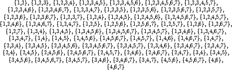
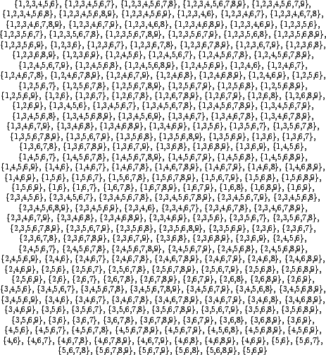
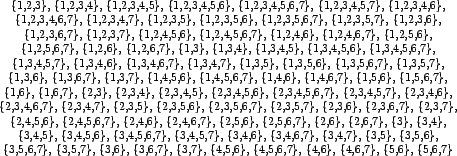
The following pages contain all directed vertex covers found for the neural networks examined in this research.